LES
More detailed results of the demonstration examples can be found in the following references:
Wall-resolved turbulent plane channel flow
This case corresponds to example/les/_manuscript_turbulent_channel.
This example simulates a fully developed turbulent plane channel flow using WRLES. The simulation employs two subgrid-scale models: the classical Smagorinsky model and the dynamic Smagorinsky model.
Domain size: (Lx, Ly, Lz) = (12.8h, 2.0h, 4.8h), where h is the channel half-height.
Boundary conditions: No-slip boundary condition in the y-direction and periodic boundary conditions in the x and z directions.
Reynolds number: Reτ = 20,000, with a friction coefficient Cf = 0.00591.
Grid resolution: Four different grids are used for a grid convergence study, with the wall-normal grid spacing varying from approximately 40+ to 10+, maintaining an aspect ratio AR = ∆x/∆z = 1.8.
The following figure shows the visualization of the turbulent channel flow obtained with WRLES:

Figure 1: Visualization of turbulent channel flow obtained with WRLES
The following figure presents the profiles of mean streamwise velocity, resolved turbulent normal stress and shear stress
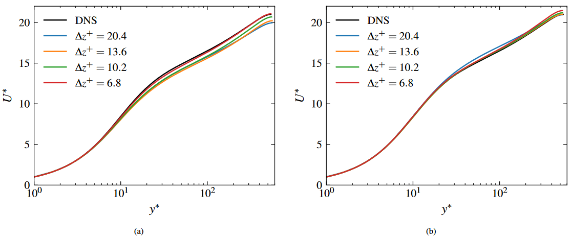
Figure 2: Mean streamwise velocity profiles with WRLES using SM (a) and DSM (b)
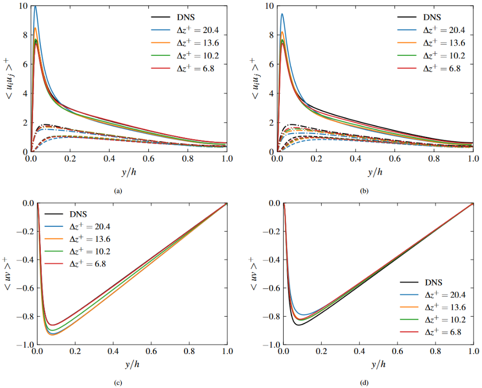
Figure 3: Resolved turbulent normal and shear stress profiles with WRLES using SM (a,c) and DSM (b,d). Line codes: ⟨uu⟩ (solid), ⟨vv⟩ (dashed), ⟨ww⟩ (dash-dotted).
Wall-modeled turbulent plane channel flow
This case corresponds to example/les/_manuscript_turbulent_channel_wall_model.
This example simulates a fully developed turbulent plane channel flow using WMLES. The simulation employs two subgrid-scale models: the classical Smagorinsky model and the dynamic Smagorinsky model.
Domain size and boundary conditions: The domain size and boundary conditions are the same as those used in the WRLES case.
Reynolds number: Reτ = 250,000, with a friction coefficient Cf = 0.00344.
Grid resolution: Thirteen different grids are used for a grid convergence study, with the wall-normal grid spacing varying from approximately 0.1h to 0.006h. The aspect ratio is AR = 1.0 and 2.0.
Wall-modeling layer thickness: The wall-modeling layer thickness is set to hwm = 0.1h.
The following figure shows the visualization of the turbulent channel flow obtained with WMLES:
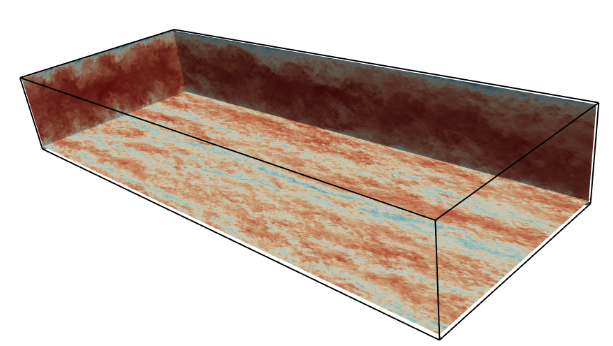
Figure 4: Visualization of turbulent channel flow obtained with WRLES
The following figure presents the profiles of mean streamwise velocity, resolved turbulent normal stress and shear stress
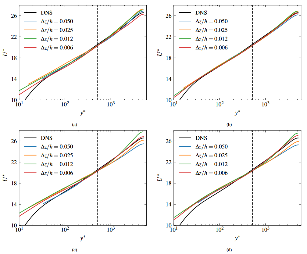
Figure 5: Mean streamwise velocity profiles with WMLES using the SM (a,c) and DSM (b,d) models on the grids with AR = 1.0 (a,b) and AR = 2.0 (c,d).
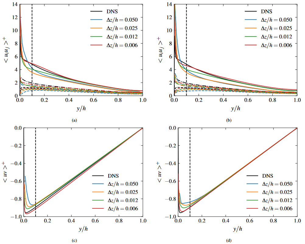
Figure 6: Resolved turbulent normal stress (a,b) and shear stress (c,d) obtained with WMLES using the SM (a,c) and DSM (b,d) models on the grids with AR = 1.0. Line codes: ⟨uu⟩ (solid), ⟨vv⟩ (dashed), ⟨ww⟩ (dash-dotted).
Wall-modeled turbulent square duct flow
This case corresponds to example/les/_manuscript_turbulent_duct_wall_model.
This example simulates a fully developed turbulent flow in a square duct using WMLES. The simulation employs two subgrid-scale models: the classical Smagorinsky model and the dynamic Smagorinsky model.
Domain size: (Lx, Ly, Lz) = (12.8h, 2.0h, 2.0h), where h is half the side length of the duct.
Boundary conditions: Wall-modeled boundary conditions are applied in the y and z directions, with periodic boundary conditions in the x direction.
Reynolds number: Reτ = 40,000, with a friction coefficient Cf = 0.00557.
Grid resolution: Six different grids are used for a grid convergence study, with the wall-normal grid spacing varying from approximately 0.1h to 0.006h.
Wall-modeling layer thickness: The wall-modeling layer thickness is set to hwm = 0.1h.
The following figure shows the visualization of the square duct flow obtained with WMLES:
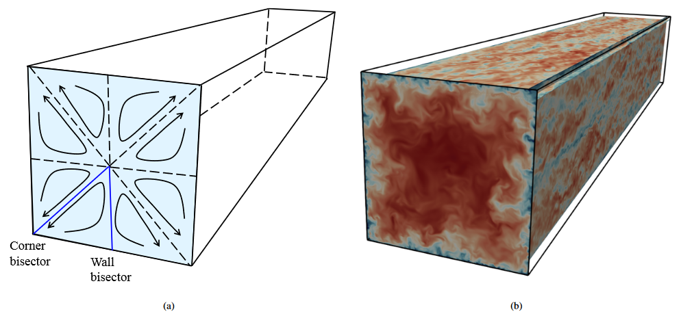
Figure 7: Visualization of turbulent channel flow obtained with WRLES
The following figure presents the profiles of mean streamwise velocity, resolved turbulent normal stress and shear stress
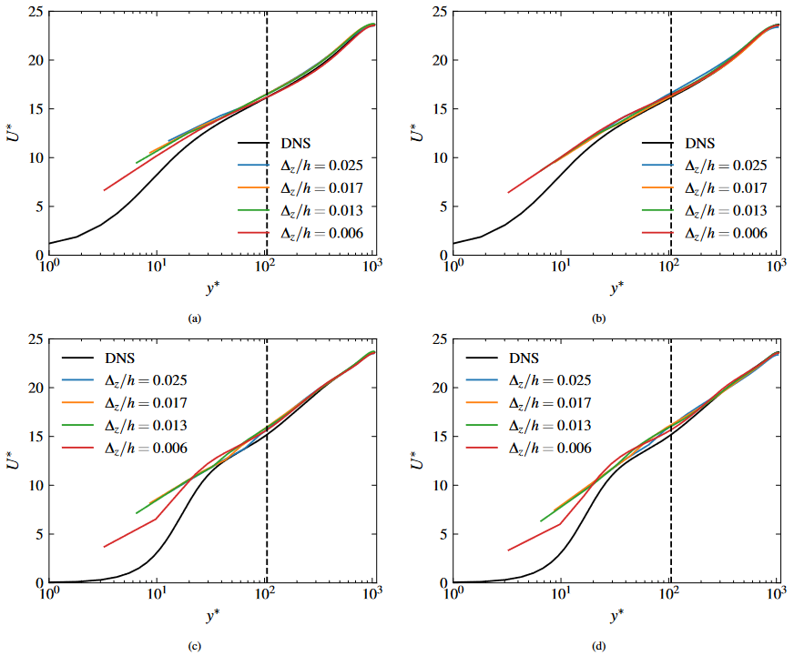
Figure 8: Mean streamwise velocity profilesalong the wall bisector (a,b) and corner bisector (c,d) obtained from WMLES with the SM (a,c) and DSM (b,d) models.
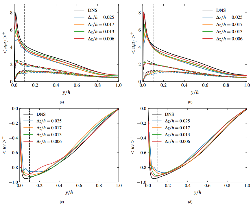
Figure 9: Resolved turbulent normal stress (a,b) and shear stress (c,d) along the wall bisector as obtained from WMLES with the SM (a,c) and DSM (b,d) models. Line codes: ⟨uu⟩ (solid), ⟨vv⟩ (dashed), ⟨ww⟩ (dash-dotted).