DNS
More detailed results of the demonstration examples can be found in the following references:
Lid-driven cavity flow
This case corresponds to example/dns/_manuscript_lid_driven_cavity.
This example simulates a lid-driven cavity flow in a cubic domain, where the top wall moves with a constant velocity while the other walls are stationary with no-slip boundary conditions.
Domain: A cubic domain with dimensions [-h/2, h/2]^3.
Boundary Conditions:
No-slip and no-penetration conditions on all walls except the top.
The top wall moves with a velocity u(x, y, h/2) = (U, 0, 0).
Reynolds Number: Defined as Re = Uh/ν = 1000.
The following figure shows the profiles of the steady-state solution at the centerlines:
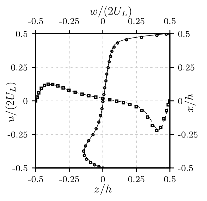
Figure 1: Profiles of the steady-state solution at the centerlines
Pressure-driven turbulent channel and square duct flow
These cases correspond to example/dns/_manuscript_turbulent_channel and example/dns/_manuscript_turbulent_duct.
This example considers two turbulent wall-bounded flows: a plane channel and a square duct. Both flows are driven by pressure and share similar boundary conditions and physical parameters.
Boundary conditions:
Both flows are periodic in the streamwise (x) direction.
No-slip/no-penetration boundary conditions are applied at the wall-normal directions:
For the square duct, at y = ±h and z = ±h.
For the plane channel, at z = ±h, with periodicity in the spanwise direction y.
Volume force: A volume force is added to the discretized momentum equation to maintain a bulk streamwise velocity Ub = 1.
Reynolds number: The Reynolds number is defined as Re = Ub(2h)/ν, with h being the channel or duct half-height
For the square duct, Re = 4410.
For the plane channel, Re = 5640.
The following figure shows the visualization of the pressure-driven turbulent channel and square duct flow:
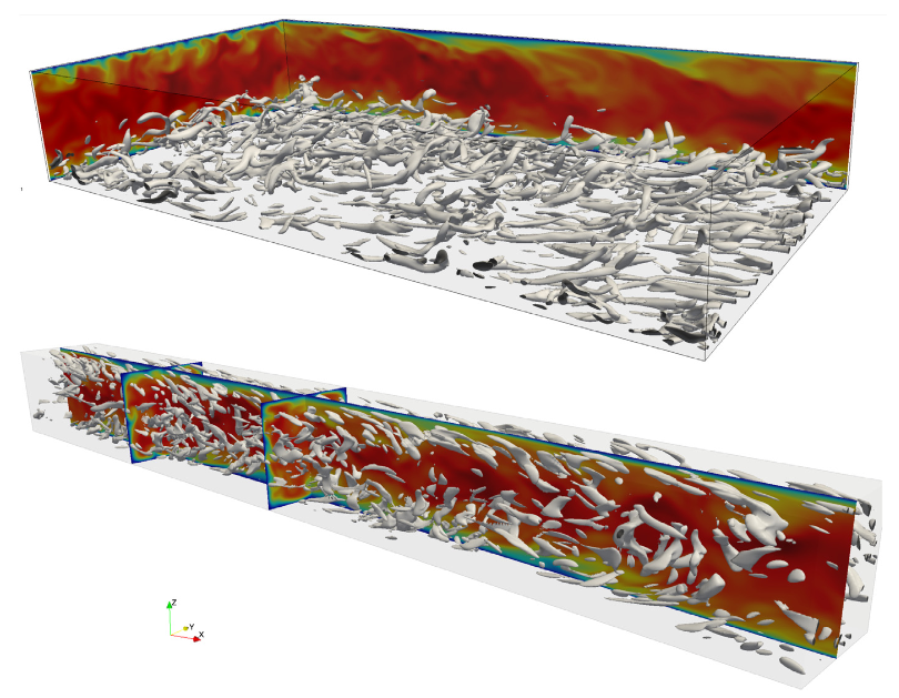
Figure 2: Visualization of pressure-driven turbulent channel and square duct flow
The following figure presents the results for the two cases:
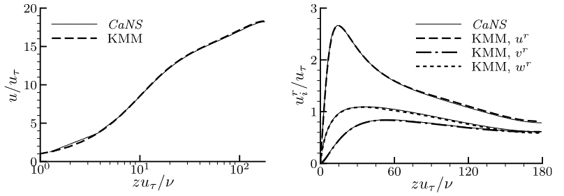
Figure 3: Mean streamwise velocity (a) and root-mean-square velocity (b) for turbulent channel flow
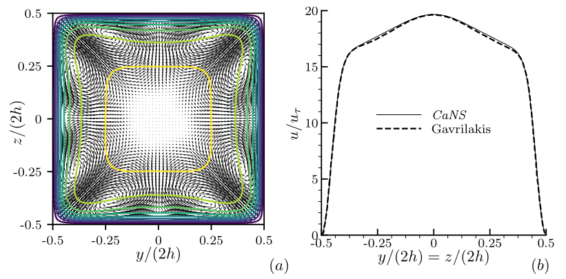
Figure 4: Mean flow (a) and mean streamwise velocity along the duct diagonal(b) for turbulent square duct flow
Taylor–Green vortex
This case corresponds to example/dns/_manuscript_taylor_green_vortex.
The Taylor–Green vortex is solved in a tri-periodic domain with dimensions [0, 2π]³. The initial velocity field is defined as:
Initial velocity field:
u0 = U sin(x/L) cos(y/L) cos(z/L)
v0 = -U cos(x/L) sin(y/L) cos(z/L)
w0 = 0
Reynolds number: The Reynolds number is defined as Re = 1600
The following figure shows the visualization of the pressure-driven turbulent channel and square duct flow:
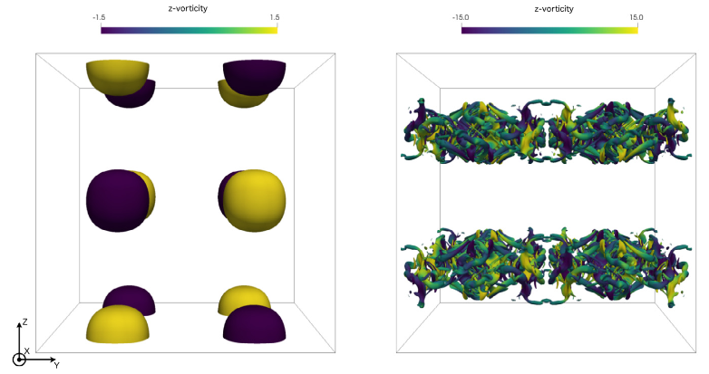
Figure 5: Visualization of Taylor–Green vortex flow
The following figure presents the results for the two cases:
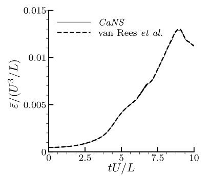
Figure 6: Mean viscous dissipation of three-dimensional Taylor–Green vortex